Selecting data based on spatial relationships#
When working with geospatial data, you often need to do specific GIS operations based on how the data layers are located in relation to each other. For instance, finding out if a certain point is located inside an area, or whether a line intersects with another line or a polygon, are very common operations for selecting data based on spatial location. These kind of queries are commonly called as spatial queries. Spatial queries are conducted based on the topological spatial relations which are fundamental constructs that describe how two or more geometric objects relate to each other concerning their position and boundaries. Topological spatial relations can be exemplified by relationships such as contains, touches and intersects (Clementini et al., 1994). In GIS, the topological relations play a crucial role as they enable queries that are less concerned with the exact coordinates or shapes of geographic entities but more focused on their relative arrangements and positions. For instance, regardless of their exact shape or size, a lake inside a forest maintains this relationship even if the forest’s boundaries or the lake’s size change slightly, as long as the lake remains enclosed by the forest. Next, we will learn a bit more details about these topological relations and how to use them for spatial queries in Python.
Topological spatial relations#
Computationally, conducting queries based on topological spatial relations, such as detecting if a point is inside a polygon can be done in different ways, but most GIS software rely on something called Dimensionally Extended 9-Intersection Model (DE-9IM [1]). DE-9IM is an ISO and OGC approved standard and a fundamental framework in GIS that is used to describe and analyze spatial relationships between geometric objects (Clementini et al., 1993). DE-9IM defines the topological relations based on the interior, boundary, and exterior of two geometric shapes and how they intersect with each other (see Figure 6.34 and Figure 6.35). When doing this, the DE-9IM also considers the dimensionality of the objects. Considering the dimensionality of geometric objects is important because it determines the nature of spatial relations, influences the complexity of interactions between objects, and defines topological rules. Typically the more dimensions the geometric object has, the more complex the geometry: The Point objects are 0-dimensional, LineString and LinearRing are 1-dimensional and Polygon objects are 2-dimensional (see Figure 6.35).
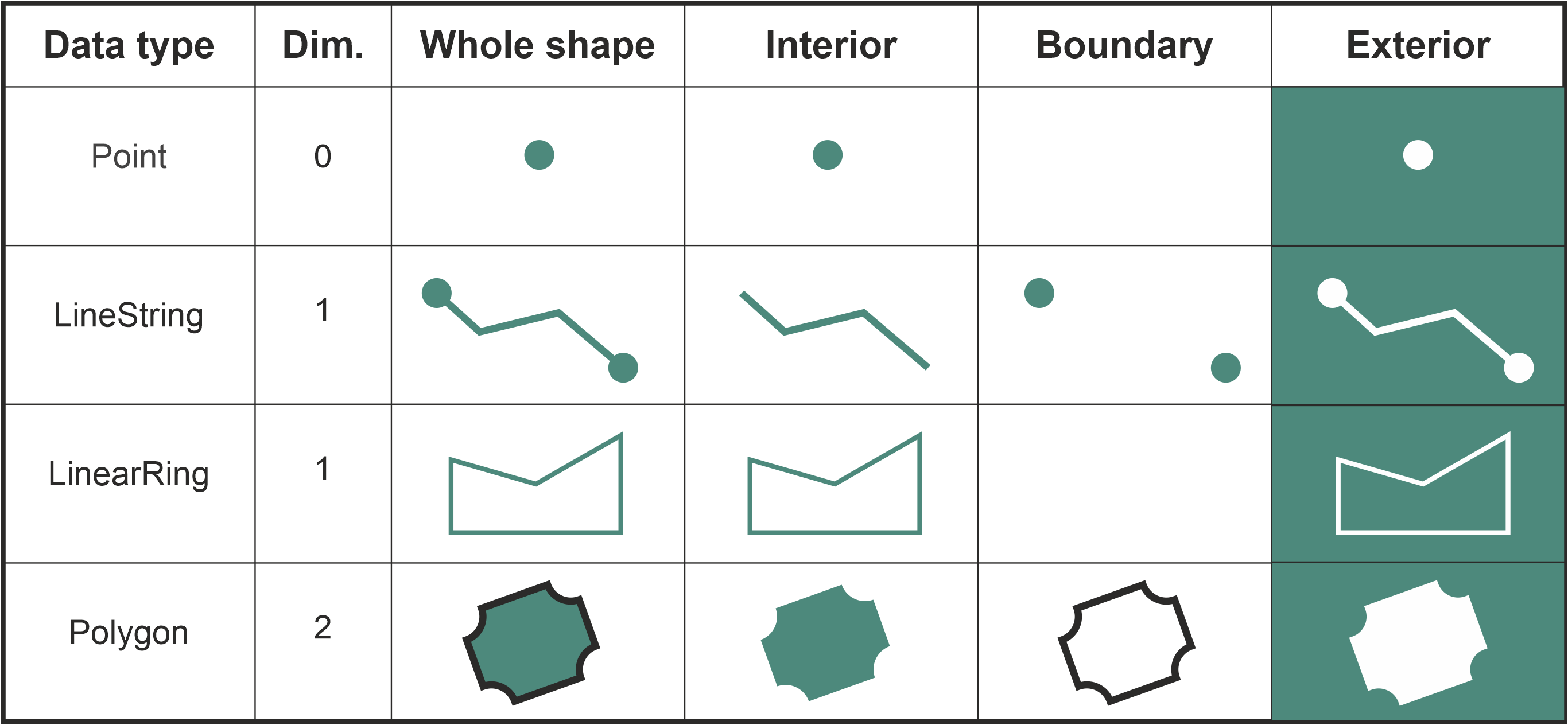
Figure 6.35. Interior, boundary and exterior for different geometric data types. The data types can be either 0, 1 or 2-dimensional.
We do not go into details about the mathematics of the DI-9IM here, but under the hood the model uses a specific 3x3 intersection matrix to examine the intersections of the interior, boundary and exterior of two geometric objects. This makes it possible to produce a detailed characterization of the geometries’ spatial relationship and one can for instance test whether a given Point or LineString is within a Polygon (returning True or False). When testing how two geometries relate to each other, the DE-9IM model gives a result which is called spatial predicate (also called as binary predicate). Figure 6.36 shows eight common spatial predicates based on the spatial relationship between the geometries (Egenhofer and Al-Taha, 1992). Many of these predicates, such as intersects, within, contains, overlaps and touches are commonly used when selecting data for specific area of interest or when joining data from one dataset to another based on the spatial relation between the layers.
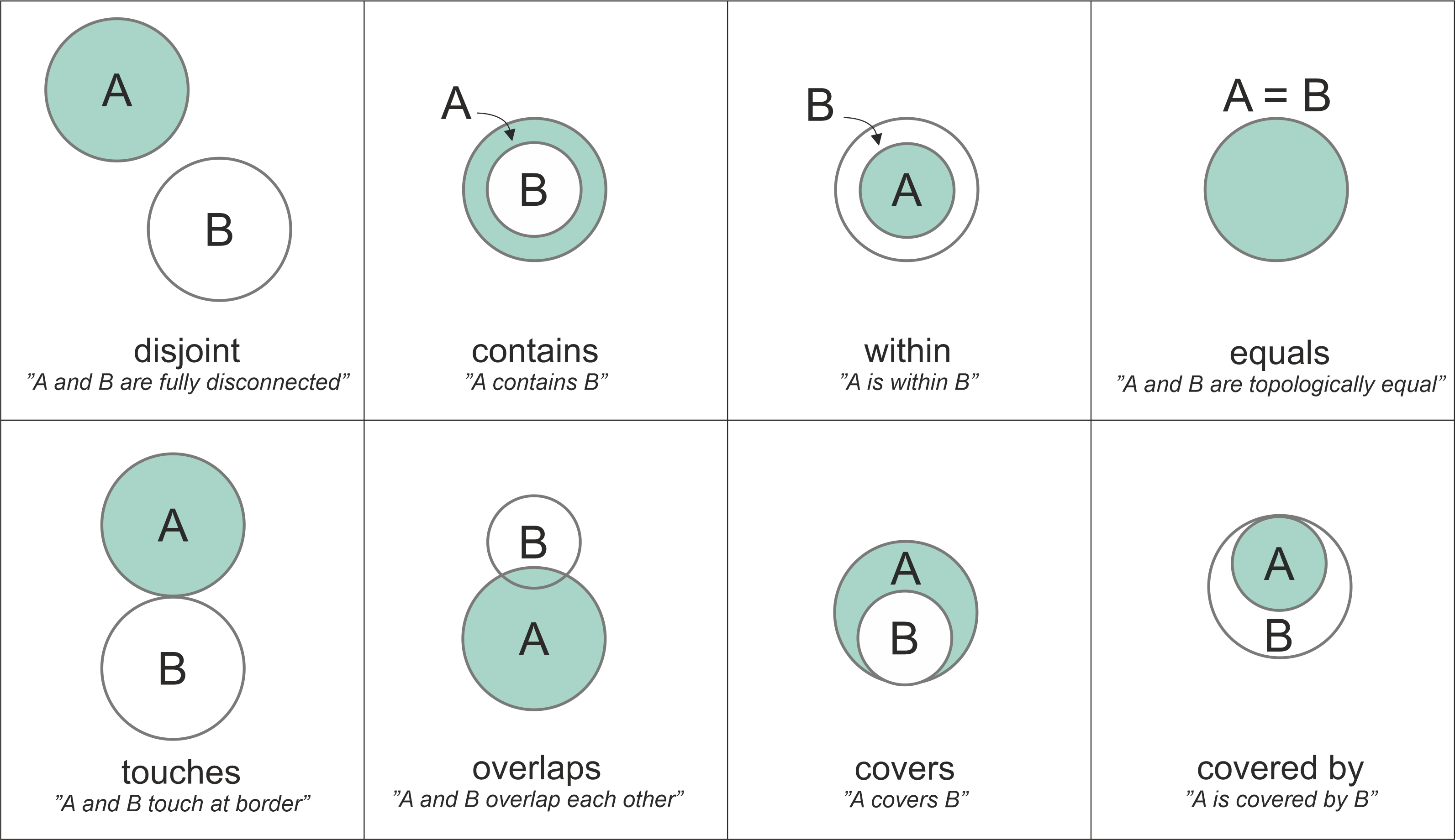
Figure 6.36. Eight common spatial predicates formed based on spatial relations between two Polygon geometries. Modified after Egenhofer et al. (1992).
The top row of Figure 6.36 shows spatial predicates in which the geometries A and B are clearly disjoint from each other, contained or within each other, or identical to each other. When the geometries have at least one point in common, the geometries are said to be intersecting with each other. Thus, in this figure, all the comparisons except the first one (disjoint) are True, i.e. the geometries intersect with each other. The bottom row shows examples of spatial relationships that are slightly “special cases” in one way or another. When two geometries touch each other, they have at least one point in common (at the border in this case), but their interiors do not intersect with each other. When the interiors of the geometries A and B are partially on top of each other and partially outside of each other, the geometries are overlapping with each other. The spatial predicate for covers is when the interior of geometry B is almost totally within A, but they share at least one common coordinate at the border. Similarly, if geometry A is almost totally contained by the geometry B (except at least one common coordinate at the border) the spatial predicate is called covered by. These eight examples represent some of the common spatial predicates based on two Polygon shapes. When other shapes are considered (e.g. Points, LineStrings), there are plenty of more topological relations: altogether 512 with 2D data.
Making spatial queries in Python#
Now as we know the basics of topological spatial relations, we can proceed and see how to make such spatial queries using Python. Luckily, we do not need to worry about the exact DE-9IM implementation ourselves, as these operations are already implemented in shapely and geopandas. With these libraries, we can evaluate the topological relationship between geographical objects easily and efficiently. In Python, all the basic spatial predicates are available from shapely library, including:
.intersects().within().contains().overlaps().touches().covers().covered_by().equals().disjoint().crosses()
When you want to use Python to find out how two geometric objects are related to each other topologically, you start by creating the geometries using shapely library. In the following, we create a couple of Point objects and one Polygon object which we can use to test how they relate to each other:
from shapely import Point, Polygon

# Create Point objects
point1 = Point(24.952242, 60.1696017)
point2 = Point(24.976567, 60.1612500)

# Create a Polygon
coordinates = [
    (24.950899, 60.169158),
    (24.953492, 60.169158),
    (24.953510, 60.170104),
    (24.950958, 60.169990),
]
polygon = Polygon(coordinates)
We can check the contents of the new variables by printing them to the screen, for example, in which case we would see
print(point1)
print(point2)
print(polygon)
POINT (24.952242 60.1696017)
POINT (24.976567 60.16125)
POLYGON ((24.950899 60.169158, 24.953492 60.169158, 24.95351 60.170104, 24.950...
If you want to test whether these Point geometries stored in point1 and point2 are within the polygon, you can call the .within() method as follows:
point1.within(polygon)
True
point2.within(polygon)
False
As we can see, the first point seem to be located within the polygon where as the second one isn’t.
One of the most common spatial queries is to see if a geometry intersects or touches another one. Again, there are binary operations in shapely for checking these spatial relationships:
.intersects()- Two objects intersect if the boundary or interior of one object intersect in any way with the boundary or interior of the other object..touches()- Two objects touch if the objects have at least one point in common and their interiors do not intersect with any part of the other object.
Let’s try these by creating two LineString geometries and test whether they intersect and touch each other:
from shapely import LineString, MultiLineString

# Create two lines
line_a = LineString([(0, 0), (1, 1)])
line_b = LineString([(1, 1), (0, 2)])
line_a.intersects(line_b)
True
line_a.touches(line_b)
True
As we can see, it seems that our two LineString objects are both intersecting and touching each other. We can confirm this by plotting the features together as a MultiLineString:
# Create a MultiLineString from line_a and line_b
multi_line = MultiLineString([line_a, line_b])
multi_line

Figure 6.37. Two LineStrings that both intersect and touch each other.
As we can see, the lines .touch() each other because line_b continues from the same node ( (1,1) ) where the line_a ends.
However, if the lines are fully overlapping with each other they don’t touch due to the spatial relationship rule in the DE-9IM. We can confirm this by checking if line_a touches itself:
line_a.touches(line_a)
False
No it doesn’t. However, .intersects() and .equals() should produce True for a case when we compare the line_a with itself:
print("Intersects?", line_a.intersects(line_a))
print("Equals?", line_a.equals(line_a))
Intersects? True
Equals? True
Question 6.8#
Use python to prove that line_a and line_b are not identical.
Following the syntax from the previous examples, we can test all different spatial predicates and assess the spatial relationship between geometries. The following prints results for all predicates between the point1 and the polygon which we created earlier:
print("Intersects?", point1.intersects(polygon))
print("Within?", point1.within(polygon))
print("Contains?", point1.contains(polygon))
print("Overlaps?", point1.overlaps(polygon))
print("Touches?", point1.touches(polygon))
print("Covers?", point1.covers(polygon))
print("Covered by?", point1.covered_by(polygon))
print("Equals?", point1.equals(polygon))
print("Disjoint?", point1.disjoint(polygon))
print("Crosses?", point1.crosses(polygon))
Intersects? True
Within? True
Contains? False
Overlaps? False
Touches? False
Covers? False
Covered by? True
Equals? False
Disjoint? False
Crosses? False
Looking at all the spatial predicates, we can see that the spatial relationship between our point and polygon object produces three True values: The point and polygon intersect with each other, the point is within the polygon, and the point is covered by the polygon. All the other tests correctly produce False, which matches with the logic of the DE-9IM standard.
It is good to notice that some of these spatial predicates are closely related to each other. For example, the .within() and covered_by() in our tests produce similar result. Also, .contains() is closely related to within(). Our point1 was within the polygon, but we can also say that the polygon contains point1. Hence, both tests produce the same result, but the logic for the relationship is inverse. Which one should you use then? Well, it depends on the situation:
if you have many points and just one polygon and you try to find out which one of them is inside the polygon: You might need to check the separately for each point to see which one is
.within()the polygon.if you have many polygons and just one point and you want to find out which polygon contains the point: You might need to check separately for each polygon to see which one(s)
.contains()the point.
Spatial queries using geopandas#
Now as we have learned how to investigate the spatial relationships between shapely geometries, we can continue and learn how to conduct spatial queries with geopandas GeoDataFrames. Conducting spatial queries with geopandas is handy because you can easily compare the spatial relationships between multiple geometries stored in separate GeoDataFrames. Next, we will run an example in which we check which points are located within specific areas of Helsinki. Let’s start by reading data that contains Polygons for major districts in Helsinki Region, as well as a few point observations that represent addresses around Helsinki that we geocoded in the previous section:
import geopandas as gpd

points = gpd.read_file("data/Helsinki/addresses.shp")
districts = gpd.read_file("data/Helsinki/Major_districts.gpkg")
print("Shape:", points.shape)
print(points.head())
Shape: (34, 4)
                                             address    id  \
0  Ruoholahti, 14, Itämerenkatu, Ruoholahti, Läns...  1000
1  Kamppi, 1, Kampinkuja, Kamppi, Eteläinen suurp...  1001
2  Bangkok9, 8, Kaivokatu, Keskusta, Kluuvi, Etel...  1002
3  Hermannin rantatie, Verkkosaari, Kalasatama, S...  1003
4  9, Tyynenmerenkatu, Jätkäsaari, Länsisatama, E...  1005

                                            addr                   geometry
0       Itämerenkatu 14, 00101 Helsinki, Finland   POINT (24.91556 60.1632)
1          Kampinkuja 1, 00100 Helsinki, Finland  POINT (24.93166 60.16905)
2           Kaivokatu 8, 00101 Helsinki, Finland  POINT (24.94168 60.16996)
3  Hermannin rantatie 1, 00580 Helsinki, Finland  POINT (24.97865 60.19005)
4     Tyynenmerenkatu 9, 00220 Helsinki, Finland  POINT (24.92151 60.15662)
print("Shape:", districts.shape)
print(districts.tail(5))
Shape: (23, 3)
           Name Description                                           geometry
18    Koivukylä              POLYGON Z ((24.99423 60.33296 0, 25.00007 60.3...
19      Itäinen              POLYGON Z ((25.03517 60.23627 0, 25.03585 60.2...
20  Östersundom              POLYGON Z ((25.23352 60.25655 0, 25.23744 60.2...
21     Hakunila              POLYGON Z ((25.08472 60.27248 0, 25.08492 60.2...
22        Korso              POLYGON Z ((25.1238 60.34191 0, 25.11997 60.34...
The data contains 34 address points and 23 district polygons. For demonstration purposes, we are interested in finding all points that are within two areas in Helsinki region, namely Itäinen and Eteläinen (‘Eastern’ and ‘Southern’ in English). Let’s first select the districts using the .loc indexer and the listed criteria which we can use with the .isin() method to filter the data, as we learned already in Chapter 3:
selection = districts.loc[districts["Name"].isin(["Itäinen", "Eteläinen"])]
print(selection.head())
         Name Description                                           geometry
10  Eteläinen              POLYGON Z ((24.78277 60.09997 0, 24.81973 60.1...
19    Itäinen              POLYGON Z ((25.03517 60.23627 0, 25.03585 60.2...
Let’s now plot the layers on top of each other. The areas with red color represent the districts that we want to use for testing the spatial relationships against the point layer (shown with blue color):
base = districts.plot(facecolor="gray")
selection.plot(ax=base, facecolor="red")
points.plot(ax=base, color="blue", markersize=5)
<Axes: >
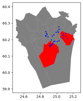
Figure 6.38. A map of Points and the two Polygon objects (in red) which we want to use for making the selection.
As we can see from Figure 6.37, many points seem to be within the two selected districts. To find out which of of them are located within the Polygon, we need to conduct a Point in Polygon -query. We can do this by checking which Points in the points GeoDataFrame are within the selected polygons stored in the selection geodataframe. In the following, we will show how to take advantage of a method called .sjoin() for doing spatial queries between two GeoDataFrames. Normally, .sjoin() method is used for conducting a spatial join between two spatial datasets, meaning that specific attribute information from a given GeoDataFrame is joined to the other one based on their topological relationship (see Chapter 6.7 for more details). However, spatial join can also be used as an efficient way to conduct spatial queries in geopandas. Consider the following example in which we use the .sjoin() method using "within" as the predicate parameter to select all points that are within the selected polygons:
selected_points = points.sjoin(selection.geometry.to_frame(), predicate="within")
ax = districts.plot(facecolor="gray")
ax = selection.plot(ax=ax, facecolor="red")
ax = selected_points.plot(ax=ax, color="gold", markersize=2)
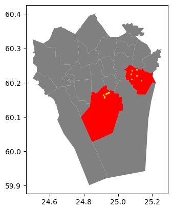
Figure 6.39. Selecting Points within red Polygons using spatial join technique.
As a result, we have now selected only the (golden) points that are inside the red polygons which is exactly what we wanted. Notice how we used the selection.geometry.to_frame() when calling the .sjoin() method. This is a special trick to avoid attaching any extra attributes from the selection geodataframe to our data, which is what .sjoin() method would normally do (and which it is actually designed for). As we are only interested in the geometries of the right-hand-side layer to do the selection, calling the .geometry.to_frame() will first select the geometry column from the selection layer and then converts it into a GeoDataFrame (which would otherwise be a GeoSeries). An alternative approach for doing the same thing is to use selection[[selection.active_geometry_name]], which also returns a GeoDataFrame containing only a column with the geodataframe’s active geometry.
In a similar manner, we can easily use the .sjoin() with other predicates to make selections based on how the geometries between two GeoDataFrames are related to each other. By default, the .sjoin() uses "intersects" as a spatial predicate, but it is easy to change this. For example, we can investigate which of the districts contain at least one point. In this case, we make a spatial join using the disctricts GeoDataFrame as a starting point, join the layer with the points and use the "contains" as a value to our predicate parameter:
districts_with_points = districts.sjoin(
    points.geometry.to_frame(), predicate="contains"
)
ax = districts.plot(facecolor="gray")
ax = districts_with_points.plot(ax=ax, edgecolor="gray")
ax = points.plot(ax=ax, color="red", markersize=2)
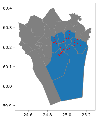
Figure 6.40. Polygons that contain at least one Point object.
As a result, we can now see that all the polygons marked with blue color were correctly selected as the ones which contain at least one point object. One important thing to remember whenever making spatial queries is that both layers need to share the same Coordinate Reference System for the selection to work properly. A typical reason for getting incorrect results when selecting data (likely an empty GeoDataFrame) is that one data layer is e.g. in WGS84 coordinate reference system whereas the other one is in some projected CRS, such as ETRS-LAEA. If this happens, you can easily fix the situation by defining and reprojecting both GeoDataFrames to same CRS using the .to_crs() method (see Chapter 6.4).
Following the previous examples, you can easily test other topological relationships as well, by changing the value in predicate parameter. To find all possible spatial predicates for a given GeoDataFrame you can call:
districts.sindex.valid_query_predicates
{None,
 'contains',
 'contains_properly',
 'covered_by',
 'covers',
 'crosses',
 'dwithin',
 'intersects',
 'overlaps',
 'touches',
 'within'}
As you can see, this list includes all typical spatial predicates which we covered earlier. But what is this .sindex that we use here? Let’s investigate it a bit further:
districts.sindex
<geopandas.sindex.SpatialIndex at 0x15006df70>
As we can see, the .sindex is something called SpatialIndex object. This is something that geopandas prepares automatically for GeoDataFrames and as the name implies, it contains the spatial index for our data. A spatial index is a special data structure that allows for efficient querying of spatial data. There are many different kind of spatial indices, but geopandas uses a spatial index called R-tree which is a hierarchical, tree-like structure that divides the space into nested, overlapping rectangles and indexes the bounding boxes of each geometry. The spatial index improves the performance of spatial queries, such as finding all objects that intersect with a given area. The .sjoin() method takes advantage of the spatial index and is therefore an extremely powerful and makes the queries faster (see Appendix 5 for further details). This comes very practical especially when working with large datasets and doing e.g. a point-in-polygon type of queries with millions of point observations. Hence, when selecting data based on topological relations, we recommend using .sjoin() instead of directly calling .within(), .contains() that come with the shapely geometries (as shown previously).
Question 6.9#
How many addresses are located in each district? You can find out the answer by grouping the spatial join result based the district name (see Part I, chapter 3 for a reminder on how to group and aggregate data).